This post will serve as the first in a series of posts about query execution plans. In this entry the goal is simply to understand that query execution plans exist, why they exist, and how to do basic navigation of them in SSMS.
Every time a query is executed on a SQL Server instance the server must decide how best to find the necessary data to be retrieved or modified. It’s not as simple as going to a table and returning rows. A table may have multiple indexes and the decision must be made about which, if any, is appropriate for this query. There might be multiple items in a where clause covering several tables. Which one should be calculated first? Are there tables that need to be joined? If so, what method should be used to join?
The server also needs to know how many resources to dedicate to the query.
How big is this query going to be? Is it big enough that it should be run multi-threaded? How many rows might be returned and how big are the rows? Based on that answer, how much memory should be requested to run this command?
SQL Server’s answers to those questions are saved in query execution plans. In the following demos we will explore these plans. The demos below utilize the WideWorldImporters DB that can be downloaded for free. Before moving on, here are some terms that will be used throughout the rest of this post.
Optimizer — The name of the program responsible for determining the best approach to a query and the resources required to run it.
Compile — The name of the process the optimizer runs to make these determinations.
Query execution plan — The product of compilation that records the determinations made by the optimizer, often shortened to query plan or execution plan.
Used in a sentence one might say, “I just clicked execute in SSMS so now the optimizer is going to compile a query execution plan for my statement so that it can run quickly.”
To follow along, open SSMS, create a new query window, connect to WideWorldImporters, and paste the following code the window.
--Query 1, A simple query looking for invoices belonging to one customer.
SELECT
 CustomerID
,InvoiceID
FROM
 Sales.Invoices
WHERE
 CustomerID = 890

--Query 2, Another simple query looking for invoices packed by a single person.
SELECT
 PackedByPersonID
,InvoiceID
FROM
 Sales.Invoices
WHERE
 PackedByPersonID = 2

--Query 3.  This query has 2 items in the where clause?  Which index should be used?
SELECT
 CustomerID
,PackedByPersonID
,InvoiceID
FROM
 Sales.Invoices
WHERE
 CustomerID = 890
  AND
 PackedByPersonID = 2
We can get a visual representation of query execution plans in SSMS and learn a lot about the queries we run. The next step is to click the “Include Actual Execution Plan” button which tells SSMS that we want to see the execution plan associated with each query we execute. Nothing should happen at this point except the color will change on that button.

At this point, highlight and execute the query 1. A new tab should now appear in the results pane next to Results and Messages. This is the Execution Plan tab. Click on that tab and the execution plan will appear. This is a very simple query and shows us a very simple plan.
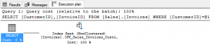
We can see that the operation performed is an index seek and that it used the [FK_Sales_Invoices_Custo…] index. That isn’t an index name for this table as the length has caused it to be cut off. We can get the entire name of that index by floating (not clicking) the mouse over the index seek operation. A new window will pop up showing the full details of the index along with a whole host of other information.
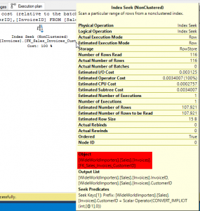
We now know that this query used the index called FK_Sales_Invoices_CustomerID. This makes sense as that index is sorted by CustomerID — the only column in the where clause. We can surmise that the optimizer didn’t have to work very hard to come up this plan.
Highlight and run the second query. This query is very similar in appearance and points to the same table as the first. The execution plan for this query looks almost identical to the first. The only difference is that the optimizer selected a different index this time, FK_Sales_Invoices_PackedByPersonID. This is an index on the column PackedByPersonID and was also an easy, but important, selection for the optimizer to make. Without the optimizer considering the differences between the selection criteria and compiling an appropriate plan this query may have run much more slowly.
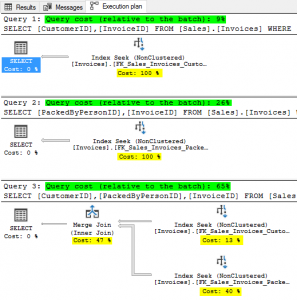
Next, we’ll examine the 3rd query. This query has selection criteria on both columns from the previous statements. Now the optimizer has a tougher decision to make. Should it use the CustomerID index or the PackedByPersonID index? After this query is executed the results are clear. It chose to use BOTH indexes and the merge the 2 result sets into a single output.
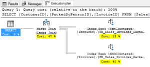
This is the first plan in this demo to include multiple steps which leads to a few more lessons about reading plans.
First, query execution plans are read right to left and bottom to top with data flowing in the direction of the arrows.
Second, the percentages assigned to each step in the plan add up to 100. These percentages are highlighted in yellow in the above screenshot. When looking at the plan of a poorly performing query one should focus on the largest percentages first as that is where SQL Server is likely spending the most effort.
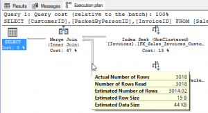
Third, the width of the arrows indicate how much data was moved from one step to the next. Floating the mouse pointer (not clicking) over the arrows shows the amount of data that was sent from one query step to the next. Floating over the widest arrow from the PackedByPersonID index shows that that seek returned 3018 rows and sent them into the merge. The slightly narrower arrow from CustomerID moved only 112 rows into the merge. And, finally, the narrowest arrow from the merge to the select carried only 10 rows, which matches the row count of the result set. We can also see an estimated row size and estimated data size in these arrows. This information is used to size the memory request to serve the query.
Finally, run all 3 queries at once. The Execution plan tab now looks a little different as it shows all 3 plans at once. In this scenario, there is another statistic that becomes useful. The optimizer will assign a percentage of overall effort for each query as related to the entire batch of queries. The 3 queries took 9%, 26%, and 65% of the effort respectively. These are highlighted in green. This does NOT alter the individual steps for each query as they still add up to 100% each as seen in yellow. If chasing down a performance issue in a query or procedure attention should first be paid to the highest percentage steps of the highest percentage queries.
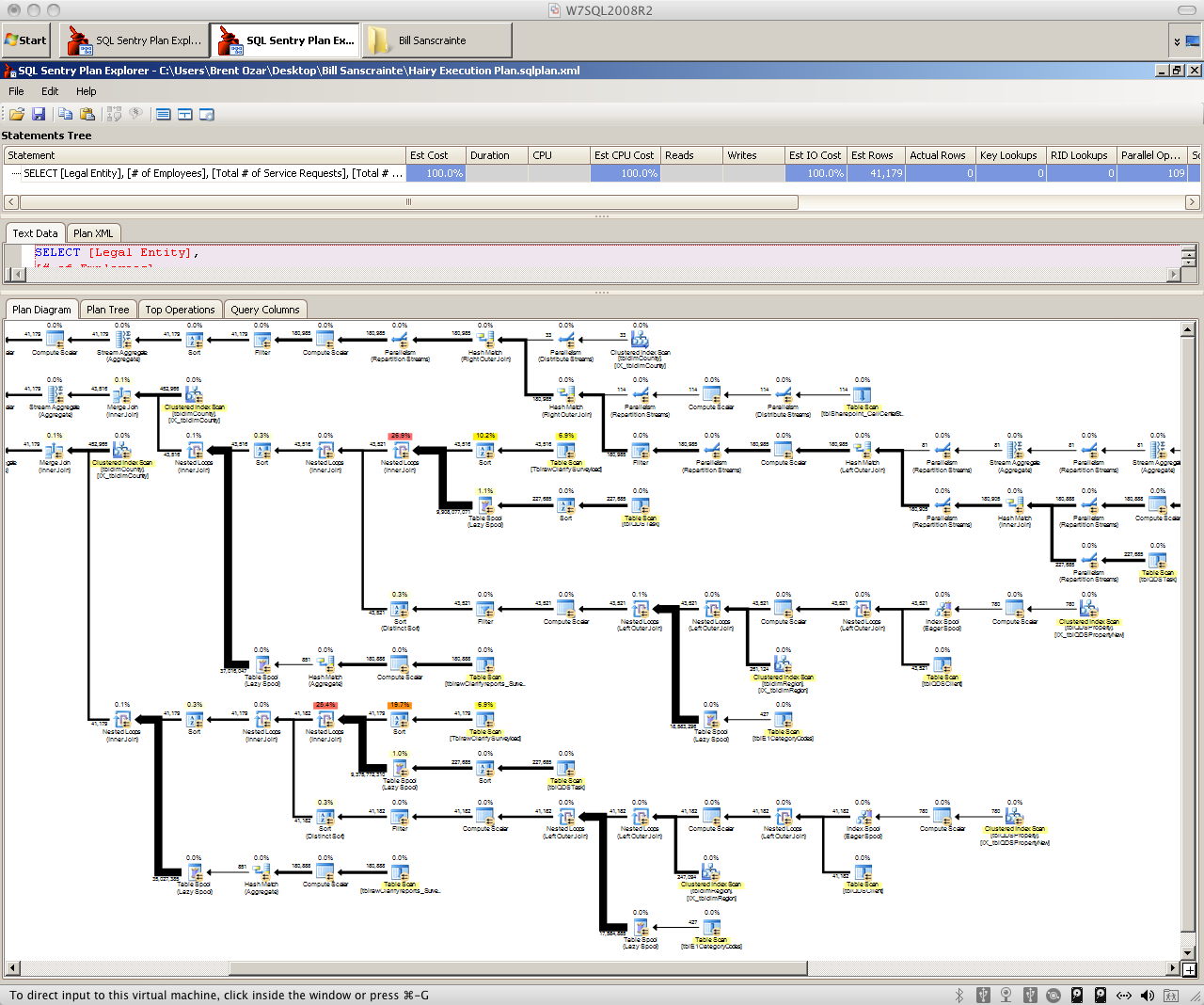
Plan can get very complicated. Learning how to read complicated plans and use the information in them to tune queries is a big time skill that takes a long time to master. It’s not something I intend to tackle in this blog. To get an idea of just how big of an undertaking this is, Grant Fritchey wrote this 300+ page book on reading execution plans. As of this writing the eBook version of Grant’s work is available for free from Red-Gate using that link. Hint Hint.
Hopefully this primer has explained what a query execution plans are, why they are important, and general navigation of plans in SSMS. I would encourage every SQL writer to build upon this knowledge and become experts at all the things Query Execution Plans can teach us about query performance.
The next entry in this series will cover how SQL Server stores and reuses these plans.